
Picture this: you're running a booming online coffee shop. If you order a small batch of beans every day, you're getting killed on shipping fees and the time it takes to process all those orders. But if you buy a year's worth of beans at once? Your cash is tied up, and you're risking a warehouse full of stale, unsellable product.
The Economic Order Quantity (EOQ) is the formula that finds that perfect sweet spot. It's designed to give you the ideal order size that keeps your total inventory costs as low as possible.
At its core, the Economic Order Quantity (EOQ) is a surprisingly simple calculation built to solve a huge problem for any ecommerce business: "How much product should I order at one time?"
The goal here is to perfectly balance two major, competing costs: ordering costs and holding costs.
Think of these two expenses as sitting on opposite ends of a seesaw. When one goes up, the other goes down.
EOQ is the mathematical magic that finds the exact point where the seesaw is perfectly balanced—the point where the sum of your ordering and holding costs is at its absolute minimum. Getting this right means you stop wasting money on endless shipping fees and stop paying to store inventory that's just gathering dust.
The classic EOQ formula elegantly pulls together three key numbers from your business to spit out an order quantity you can actually use. Getting a handle on these variables is the first step to putting this powerful tool to work.
The real genius of the EOQ model is its simplicity. It boils down a complex inventory puzzle to the fundamental trade-off between placing an order and holding the stock. For merchants, it’s the first step away from gut-feel ordering and toward a truly data-informed strategy.
Developed by Ford W. Harris way back in 1913, the standard formula has remained a cornerstone of inventory management for over a century. Its staying power comes from its square root relationship, which creates a cost curve that bottoms out at the perfect order quantity. For modern D2C brands, this old-school principle is as relevant as ever because that core tension between ordering and holding costs is timeless. You can learn more about the history and impact of this foundational inventory formula.
To get started, you just need to nail down three figures:
To make this crystal clear, here’s a quick breakdown of each component in the EOQ formula.
| Variable | What It Represents | Example for a Shopify Store |
|---|---|---|
| D | Annual Demand | The total number of "Organic French Roast" coffee bags you sold last year. Let's say it's 1,200 bags. |
| S | Ordering Cost | The cost per purchase order. This includes staff time ($10), payment processing fees ($2), and standard shipping ($8), for a total of $20 per order. |
| H | Holding Cost | The cost to store one coffee bag for a year. Includes warehouse space ($1.50), insurance ($0.25), and potential spoilage ($0.25), totaling $2.00 per unit. |
With these three variables in hand, you have everything you need to plug into the formula and find your magic number.
To really get a handle on the Economic Order Quantity, you have to look past the math for a second. The magic isn't in plugging in numbers; it's in understanding the elegant push-and-pull the formula solves. Think of it as finding the sweet spot where your total inventory expenses are at their absolute lowest.
At its core, the EOQ model is a balancing act between two competing costs: how much it costs you to order products versus how much it costs you to hold them. These two forces are always working against each other.
If you place small, frequent orders, your warehouse shelves stay lean and your holding costs are low. Great, right? Not entirely. You end up paying a ton in ordering costs from all those transactions. On the flip side, buying in huge quantities means fewer orders, but now your holding costs—storage, insurance, capital—shoot through the roof.
The EOQ formula is designed to find that perfect middle ground. Let's pull apart each side of this equation.
Figuring out your total ordering cost for the year is pretty straightforward. It boils down to how many orders you place and the fixed cost you pay for each one.
Here's the simple formula: Total Ordering Cost = (D / Q) * S
The (D / Q) part just tells you how many orders you'll make. For instance, if you sell 1,200 units a year (D) and you order 100 at a time (Q), you’re placing 12 orders. If each order costs you $20 (S), your total annual ordering cost is 12 * $20 = $240. Easy enough.
This diagram helps visualize the key inputs that make the EOQ calculation work.
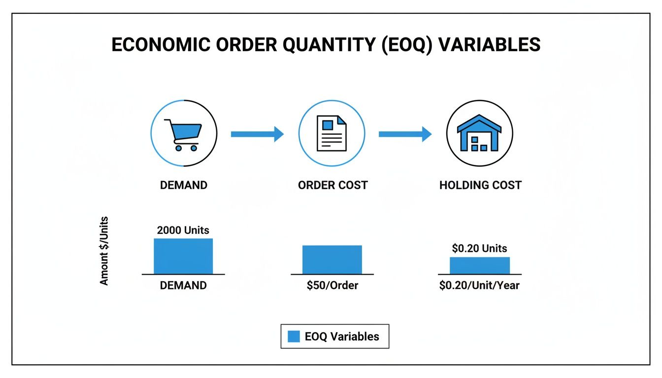
As you can see, demand, order cost, and holding cost are the three pillars of the EOQ strategy. Each one puts a different kind of financial pressure on your business, and the formula finds the balance.
Next up is the cost of simply having inventory sitting on your shelves. This is all about your average inventory level and what it costs to store one unit for an entire year.
The formula for this is: Total Holding Cost = (Q / 2) * H
Why (Q / 2)? This represents your average inventory. You start with a full shipment (Q) and sell through it until you hit zero, right before the next shipment arrives. So, on any given day, you're holding, on average, half of your order quantity.
Let's say you order 100 units (Q) and your annual holding cost per unit (H) is $4. Your total annual holding cost would be (100 / 2) * $4 = $200. To get a better grip on this number, you can dive deeper into what is inventory carrying cost and all the little expenses that make it up.
This is where it all clicks. The lowest possible total inventory cost happens at the precise point where your Total Ordering Cost equals your Total Holding Cost. That's the equilibrium we've been looking for.
By setting the two formulas equal to each other—
(D / Q) * S = (Q / 2) * H—and doing a bit of algebra to solve for Q, we arrive at the classic EOQ formula. It’s not just some random equation; it's the mathematical proof of perfect inventory balance.
When we rearrange that equation to isolate Q, we get the final result:
EOQ = √((2 * D * S) / H)
This formula gives you the ideal number of units to order (Q) that makes both sides of the cost equation equal, minimizing your total inventory expenses. Of course, to use this effectively, you need to know how to accurately calculate cost per unit, since that number is a key building block for both your demand and holding cost figures.
All the theory in the world doesn't mean much until you see how it plays out with real products. This is where the Economic Order Quantity formula really clicks—when you plug in actual numbers and see how different types of products demand completely different ordering strategies.
To make this tangible, we'll walk through two classic scenarios for any direct-to-consumer brand. First up, a high-volume, low-cost wellness supplement. Then, we'll look at a lower-volume, higher-cost consumer electronic device.
Let's say you're selling a popular "Daily Greens" powder. It's a steady seller, and the unit cost is low, which means your holding costs are pretty manageable. Here are some realistic numbers we can work with:
Now, let's plug these into the EOQ formula:
EOQ = √((2 * D * S) / H)
EOQ = √((2 * 20,000 * $50) / $1.50)
EOQ = √($2,000,000 / $1.50)
EOQ = √1,333,333
EOQ ≈ 1,155 units
The math tells us the sweet spot for your order size is 1,155 units. This means you’d place about 17 orders per year (20,000 / 1,155) to keep your total inventory costs as low as possible. Ordering this amount perfectly balances what you spend on placing orders with what you spend on storing the product.
Next, let's switch gears to a pair of premium noise-canceling headphones. Demand is consistent but much lower than the supplement, and because each unit is expensive, your holding costs are a much bigger deal.
Putting these numbers into the same formula gives us a wildly different result:
EOQ = √((2 * D * S) / H)
EOQ = √((2 * 800 * $50) / $40)
EOQ = √($80,000 / $40)
EOQ = √2,000
EOQ ≈ 45 units
For the headphones, the EOQ is just 45 units. This works out to placing around 18 orders per year (800 / 45)—a similar frequency to the supplement, but for a tiny fraction of the volume. Why? The steep holding cost heavily penalizes you for carrying extra stock, forcing the optimal order size way down.
These examples prove that EOQ isn't some magic number you find once and apply everywhere. It’s a dynamic tool that adapts to each product’s unique financial DNA, saving you from using a single, inefficient ordering rule for your whole catalog.
Take another common scenario: a clothing brand sells 1,000 skirts annually with a $5 holding cost and a $2 ordering cost. Their EOQ would be around 63 units, meaning they should place about 16 orders per year. These real-world calculations show why D2C brands can’t just rely on gut feel. If you're curious to see more breakdowns, Bizowie's piece on how the EOQ formula provides a complete guide to optimal inventory ordering is a great resource.
The contrast between our supplement and headphone examples really stands out when you put them side-by-side. The math is the same, but the inputs completely change the final strategy.
| Variable | Example 1 Wellness Supplement | Example 2 Consumer Electronic |
|---|---|---|
| Annual Demand (D) | 20,000 units | 800 units |
| Ordering Cost (S) | $50 per order | $50 per order |
| Holding Cost (H) | $1.50 per unit | $40 per unit |
| Calculated EOQ | 1,155 units | ~45 units |
| Orders Per Year | ~17 orders | ~18 orders |
| Strategic Implication | Order in large batches to minimize frequent ordering costs. | Order in very small batches to avoid tying up capital and incurring high storage costs. |
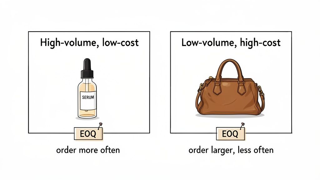
This comparison drives home the core lesson: high holding costs make over-ordering painful, pushing you toward smaller, more frequent purchases. But when holding costs are low, it's smarter to place larger orders less often to save on administrative and shipping fees.
The standard Economic Order Quantity formula is a fantastic tool. It gives you a clean, mathematical answer to the fundamental question: "How much should I order?" It works perfectly in a perfect world, but as any merchant knows, reality is a lot messier.
Suppliers will dangle tempting bulk discounts in front of you. Brands that manufacture their own goods operate on totally different replenishment cycles. To truly get a handle on your inventory, you need to adapt the EOQ concept to these common situations. Let's look at two critical variations that take the core logic of EOQ and apply it to the dynamic nature of modern e-commerce.
One of the most frequent curveballs you'll face is the quantity discount. A supplier might offer a lower price per unit if you buy 500 units, even though your calculated EOQ is only 300. On the surface, it seems like a no-brainer—cheaper is better, right?
Not so fast. A bigger order means your average inventory swells, which in turn jacks up your annual holding costs. The Quantity Discount Model is how you figure out if the savings from the cheaper unit price are actually worth the increased cost of storing all that extra product.
The key here is that the purchase price itself is no longer a fixed number. The goal shifts from just balancing ordering and holding costs to minimizing the total annual cost, which now includes the cost of the goods themselves.
To work this out, you just need to follow a few straightforward steps:
This simple comparison stops you from getting suckered into a bulk deal that secretly costs you more in the long run because of bloated warehousing expenses.
The basic EOQ formula assumes your entire order magically appears in your warehouse in one big drop. For brands buying from a third-party supplier, this is often close enough to how it works. But what if you’re the one making the products?
This is where the Production Order Quantity (POQ) model (sometimes called the Economic Production Quantity, or EPQ) becomes essential. It’s built for businesses where inventory is replenished gradually over time as it’s produced, not all at once.
Imagine a bakery that makes 100 loaves of bread each day but only sells 25. Their inventory doesn't leap from zero to 100; it builds up slowly as loaves come out of the oven. The POQ formula accounts for this gradual increase by factoring in both the daily production rate and the daily demand rate. This keeps you from overestimating your average inventory levels and the holding costs that come with them.
You can learn more about how this fits into broader inventory reorder strategies that go beyond simple purchasing. The POQ model helps vertically integrated brands fine-tune their production runs to minimize the costs of both machine setup (the manufacturing version of ordering costs) and warehousing finished goods.
It also connects to other vital metrics. For instance, knowing how to calculate safety stock is even more critical when your replenishment isn't instant. These adapted EOQ formulas give you a much sharper, more accurate picture for managing inventory outside the simple buy-and-sell model.
While the economic order quantity formula gives you a powerful, data-driven starting point, it's not a crystal ball. Its mathematical elegance comes from a set of simplifying assumptions that basically create a "perfect world" scenario for your inventory. But as any Shopify merchant knows, we don't live in a perfect world—we live in one full of unpredictable sales and supply chain curveballs.
Understanding the model's built-in limitations is the key to using it intelligently. It helps you know when to trust the number it spits out and when to treat it as a strategic baseline that needs a healthy dose of real-world adjustment.
The classic EOQ model operates on a foundation of total predictability and consistency. It has to assume several conditions are always true, which can be a huge departure from the day-to-day realities of running an online store.
The main assumptions include:
The EOQ formula is a snapshot taken in a perfectly stable environment. It provides an optimal answer for a business that never changes. The real skill lies in using that snapshot as a guidepost while navigating the constant motion of your actual market.
These assumptions can create a major gap between theory and what actually happens on the ground, especially in fast-moving D2C sectors.
The EOQ model is built for a world where demand never wavers, stock arrives instantly, and costs are fixed. But in today's retail markets—especially for Shopify merchants in competitive niches like health, fashion, and electronics—demand is anything but stable. It’s influenced by seasonal trends, marketing campaigns, and random market disruptions. If you're managing hundreds of SKUs, applying a simple EOQ formula without thinking about how products relate to each other or how much warehouse space you actually have can lead to some seriously subpar results. You can find more insights on navigating these ecommerce inventory challenges on Logiwa.com.
For example, a sudden 40% surge in demand from a holiday sale completely blows the "constant demand" assumption out of the water. If you ordered based on a rigid EOQ calculation, you'd stock out in no time. Similarly, if a key supplier has a production hiccup, the "instant replenishment" assumption breaks down, leaving you with empty shelves and frustrated customers.
This doesn't mean the EOQ formula is useless. Not at all. It just means you have to see it for what it is: a foundational tool, not a complete inventory management system. It brilliantly solves for the cost balance between ordering too much and ordering too often, giving you a crucial piece of the puzzle. The next step is to layer this insight with other tools—like safety stock calculations and modern forecasting software—to handle the volatility the basic formula ignores.
The core ideas behind the economic order quantity formula are timeless, but the tools we use to put them into practice have come a long way. While scribbling out EOQ calculations on a spreadsheet gives you a solid baseline, modern inventory platforms are built to move beyond static numbers and deliver smart recommendations that actually reflect the chaos of real-world business.

Instead of just plugging in a single, fixed number for your annual demand, these systems dig into your live sales data. They're designed to spot the subtle trends and seasonal shifts that the classic formula was never built to see, turning a historical snapshot into a forward-looking forecast.
Tools like Tociny.ai don't throw out the EOQ logic of balancing ordering and holding costs—they supercharge it with live data streams. They stop asking, "What was last year's demand?" and start continuously analyzing and predicting future demand with much greater accuracy.
This isn't just a small tweak; it's a completely different approach that juggles multiple variables at once: * Real-Time Sales Velocity: It tracks how fast a product is selling right now, not just its yearly average. * Seasonality and Trends: It automatically detects predictable peaks (like Black Friday) and adjusts for emerging trends without you having to lift a finger. * Supplier Lead Times: It factors in your suppliers' current performance to fine-tune reorder points on the fly. * Promotional Impact: It learns from past marketing campaigns to anticipate demand spikes during your next big sale.
By plugging into live data, modern software transforms EOQ from a simple math problem into a responsive, living inventory strategy. It stops you from ordering based on last year's news and starts aligning your stock levels with what’s actually happening in your business today.
The real magic here is moving from a single "optimal" number to a holistic inventory plan. Instead of you manually crunching EOQ numbers for hundreds of SKUs, an AI-powered platform can generate adaptive recommendations that keep you from stocking out on winners and overstocking on duds.
It essentially takes the foundational wisdom of EOQ and puts it on autopilot. If you want to dive deeper, you can explore the various modern inventory optimization techniques that build on these classic ideas.
This shift frees you up from the drudgery of endless spreadsheets, letting you focus on big-picture strategy instead of tedious calculations. The result is a leaner, more profitable inventory system that's always one step ahead of your customers.
Even after you've got the formulas down, you're bound to have some practical questions when it's time to actually use EOQ in your business. Let's walk through some of the most common hurdles merchants face when moving from theory to reality.
Getting a handle on your costs is the most important step here. The formula is only as good as the numbers you plug into it. Don't chase perfection—a solid, well-reasoned estimate is miles better than a wild guess.
Start by breaking down the two main cost buckets:
For a smaller business, you might find that $25 in staff time and fees (S) and $3.50 in annual storage per unit (H) are perfectly reasonable starting points.
This trips a lot of people up, but the distinction is actually pretty simple once you see how they work together to create a full inventory control system. They just answer two different—but equally critical—questions.
The EOQ formula tells you 'how much' to order. The reorder point (ROP) tells you 'when' to place that order.
In the real world, your reorder point acts as a trigger. When your stock on hand for a product drops to your predetermined ROP, that's your cue to place a new order for the quantity your EOQ calculation gave you. This one-two punch ensures you order the most cost-effective amount at exactly the right time to dodge stockouts.
Here’s where the classic EOQ formula shows its age. Its biggest weakness is that it assumes demand is steady and constant all year long. For products with big seasonal swings—like swimsuits in the summer or holiday decor in the winter—a single, year-round EOQ is a recipe for disaster. You'll be sold out during your peak season and drowning in excess inventory during the off-season.
But you can still adapt the underlying principle. The simplest workaround is to calculate different EOQs for different times of the year. For instance, you could figure out one EOQ for your busy season (say, May-August) and a totally separate one for your slower months (September-April), using the specific demand forecast for each of those periods.
Ultimately, though, for products with highly variable demand, modern inventory tools are a much better bet. They automatically adjust for seasonality and trends, using the same core logic of balancing costs but applying it to a dynamic, forward-looking forecast instead of a flat, static annual number.
Ready to move beyond static formulas and get real-time inventory recommendations? Tociny.ai replaces tedious spreadsheet calculations with AI-powered forecasting, helping you optimize stock levels and make smarter, data-driven decisions. Discover how at https://tociny.ai.
Tociny is in private beta — we’re onboarding a few select stores right now.
Book a short call to get early access and exclusive insights.